Infratech Civil

Product:  Autodesk SSA  |   Subject: Storm and Sanitary Analysis

---

In this exercise, we will learn about SSA Interface.

SSA User Interface

Now that we have the design background data imported from Civil 3D, one might think that we should start designing right away.  While that’s true, we are going to pump the brakes just a little bit and discover the SSA interface first. We need to acquaint ourselves with the tools available to us for the detailed design.

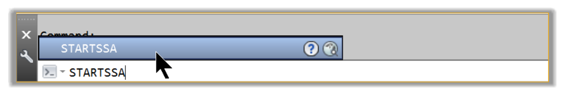
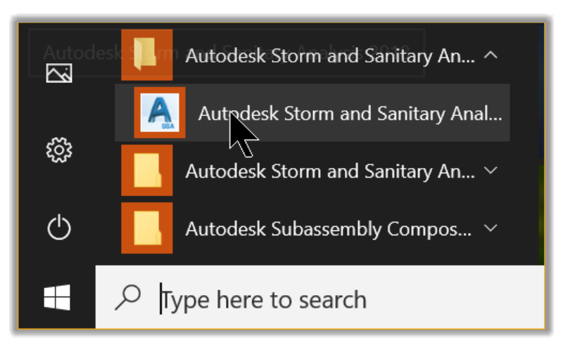
In this chapter, we will peruse the user interface and discover the essential features and commands of SSA. We already saw how to launch SSA by exporting a Civil 3D pipe network. However, we can also launch SSA by using several other options, including:

1. The Civil 3D ribbons.

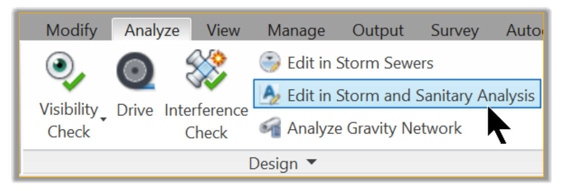
2. Typing StartSSa at the command line of Civil 3D;

3. The SSA shortcut from the Windows programs menu.

4. Or simply double-click an existing project file (SFP format).

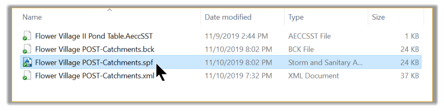
If you already have the SSA – POST-Catchments file opened, keep working with the same file. If not, you can launch the following file from the practice Model folder: 03.01-SEWERS-Interface-General.spf

SSA is now opened. We can see the user interface. The major elements of the user interface include the following components:

1. Plan View
2. Menu Bar
3. Data Tree
4. Toolbars
5. Status Bar
6. View Tabs

Now, let's explore these items in more details. 

SSA Plan View

This is where we see the different components of the stormwater or the sanitary sewer network. This is also where we can layout the system if it was not already imported from Civil 3D. In the plan view we can:

1. Create a schematic of different elements of the network (in real or unscaled distances). 
2. Provide a color-coded display of the properties of the different elements making up the system. We can display them proportional to their values (peak flows, velocities, sub-basin runoffs, structure water levels, and more)
3. Adjust the network manually to select, reposition, delete, or add new elements. Elements can also be imported from files such as LandXML, GIS, AutoCAD, or other modeling software like SWMM and others).
4. Overlay background information such as maps, aerial imagery, Geo-referenced TIFF, AutoCAD base drawings, etc.
5. Browse the drainage network by zooming to different areas or the extent of the project.
6. Display Channels and pipes flow arrow directions.
7. Annotate element with data labels or IDs.
8. Display profile views of pipe runs and generate reports of the stormwater analysis.

Project Data Tree

The Project Data Tree is the column to the left if the SSA interface. It allows us to access the data for most elements in a project.

We can access the data for any particular element by double-clicking on it in the Data Tree.

For example, clicking on Junctions in the data tree will display a window with the data for all the nodes included in the project.

We can expand and collapse it by simply double-clicking on Project Data at the top of the tree.   In the data tree, the elements are organized in a hierarchical and logical order, from the top down. It’s logical because when working on a project, it makes sense that we start by specifying the project Options, then the Analysis Option, the hydrology data, and the hydraulics information. If water quality is required, we can then do that and work on other details such as Control Rules, Sanitary Patterns, and Time Series. As a matter of fact, we use this top-down design approach in most of our projects.

One last thing we need to note about the Data Tree is that its content is dynamic and adjusts depending on the project options. For example, if a project is running a Rational Method hydrologic model, the Data Tree, will adjust to show an IDF input option. On the other hand, a project with a SWMM model option will display a rain gage option, so the user can input historical rainfall time-series information.

Let’s explore some of the lines in the Data Tree. First, the Project Options.  

3.1.2.1                Project Options

The Project Options is the first line in the data tree. The Project Options dialog box contains a tabbed interface, allowing us to click the tab of interest to see the data defined within the tabbed pane.

1. First, let’s double-click on Project Options.

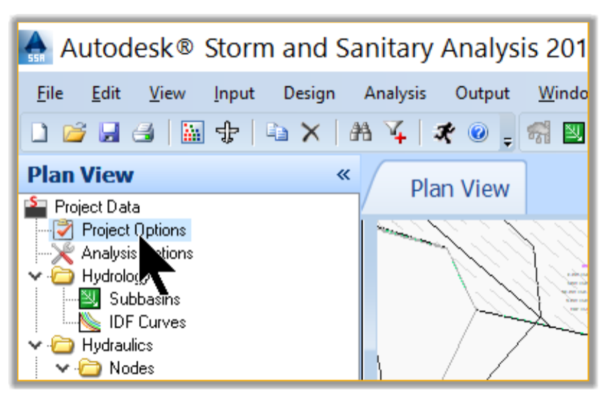
2. This will display the options for the project.

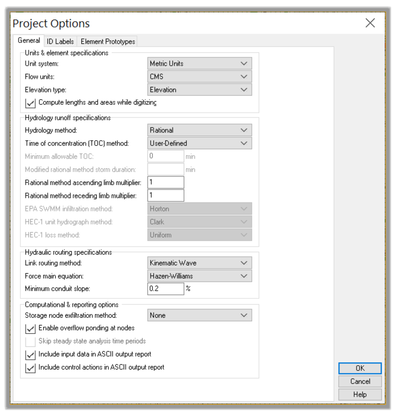
3. This is typically one of the first steps in an SSA project. We need to specify the design options. We have tabs that allow us to specify different design options and parameters:
   1. First, the General tab: it allows us to specify various settings of the model, such as the project units (international or imperial), the hydrologic model for runoff generation. In the Options windows here, we need to make sure we are choosing the right units for our project (Metrics or US), depending on our location. Then, the most important parameter here is the Hydrology Method. Among the options we have some of the most widely recognized hydrological models such as HEC-1, EPA-SWMM, SCS TR-55, the Rational Method, and its modifications, etc. Depending on the hydrologic method chosen, we have a different time of concentration options such as FAA, Kirpich, SCS TR-55 or User-Defined. Let’s choose the Rational Method. It is one of the most accepted methods for underground pipe design. There are typically two main components of the stormwater design we need to consider:

      The first one is the sewer system, which is designed with the 10-Year storm event. This means the pipes and structures should not be surcharged during the 10-year storm event.

      The detention design, where we should make sure our post-development peak flow should be equal or less than the pre-development during the 100-Year storm event. 

So, we have two parallel designs going on. The first one is for the piping system, which should carry the 10-year flow without any flooding on the street. The Rational method is usually the best method for this condition.

The second is for the 100-year, where the pond should act as a buffer to throttle the maximum off-site flows to pre-development levels. For this model, usually, we will use the EPA SWMM, TR-55 or the Modified rational, which is an extended Rational method. The reason for this is because detention calculations are required over an extended period of time, typically 24-Hours. On the other hand, the peak flows for the sewers usually happen during the first 10 to 15 minutes for small sites. That makes the Rational method suitable for this calculation because it uses an IDF curve with the highest intensities in the 5 to 10 minutes timeframe.

On this tab, we can also specify the hydraulic routing method. Our options are the steady flow, kinematic wave, or hydrodynamic method. Generally, we will always recommend the hydrodynamic method, because it is a complete hydraulic routing method. It solves the complete St Venant equation, which works for steady flows, reverse, or backwater conditions since it allows for the conservation of momentum. However, we must be aware that this method requires a much smaller time step than the Kinematic Wave Routing and Steady Flow Routing methods. The Kinematic and Steady flow methods are fine when we have simple projects where no backwater conditions are expected. Typical values for a Hydrodynamic Routing time step range from 60 seconds to 1 second. The smaller the time step, the more accurate the computations of the peak flow values.

2. On the ID Labels tabs, we have options for specifying the default naming prefixes and suffixes digits and increments.
3. The last tab, Element Prototypes, allows us to determine the default values of the elements such as areas, widths, slopes, coefficients, elevations, heights, depths, geometries, diameters, etc. Obviously, these default values will be replaced by the real project values, if required, at any time during the modeling process.

4. To recap for the project options, in the next chapters, we have two designs and will choose different parameters for each one. 

SSA Analysis Options

The next item after Project Options in the data tree is “Analysis Options.”

1. Click on the Analysis Option under the Data Tree.

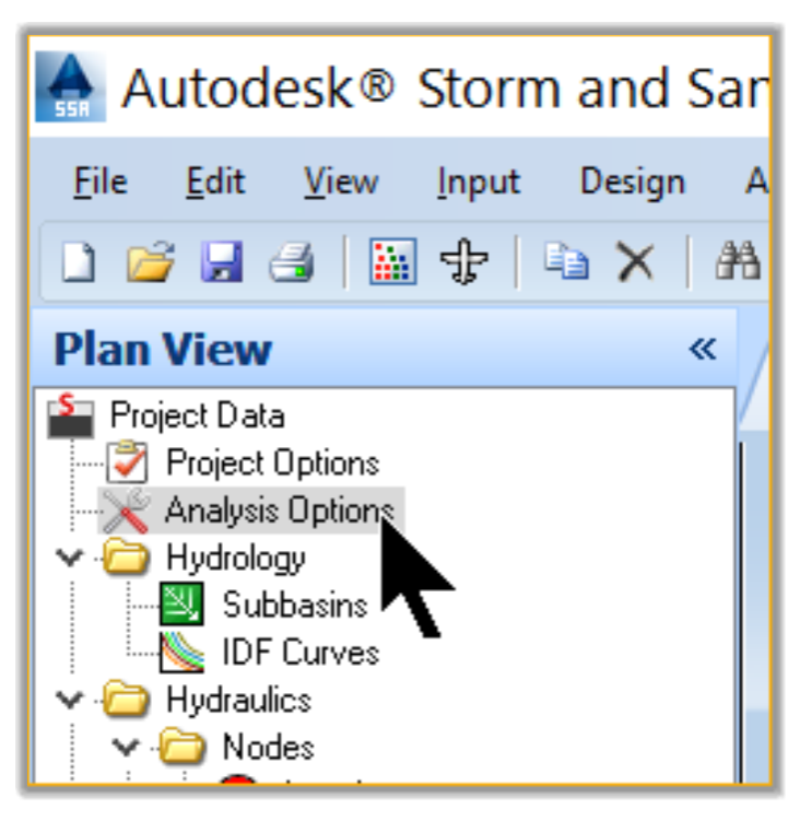
2. In this window, we have two tabs. The first one, General, allows us to assign the general settings of the analysis. This includes items such as the simulation time steps, dates (start and end), and initial weather conditions, the different parameters to analyze such as runoff, flow quantities, and qualities. We can also specify the supercritical flow conditions. In general, we will leave all these values to their default. Additionally, we can also read or write external interface files. These options are mostly for large scale watersheds where we are dealing with externally imposed inputs (e.g., Rainfall or inflow/infiltration hydrographs) or where previous analyses have been done, and we want to integrate those results. This can help speed up a simulation or compare multiple scenarios. 
3. The second tab is “Storm Selection.” It allows us to define the storm or storms to be analyzed. Obviously, if the Hydrology Runoff Computational option on the General tab is unchecked, then we will have the Storm Selection tab unavailable. We can also use this tab to define either a single or multiple storm event. 

HSSA Hydrology

Up next in the data tree is the Hydrology section.  Obviously, the hydrology of a project is mainly impacted by two factors: the physical nature of the project site, represented by catchments, and the weather conditions, mostly rainfall. Depending on the hydrologic method we choose, the rainfall is input either by:

• IDF curves, which represent a relationship between the rainfall Intensity, the Duration, and Frequency.
• Or, rain gage data, which are historical recordings of rainfall.

In both cases, the analysis is done for a return period, which represents the statistical probability of a given rainfall to occur. For example, a 1:100-year frequency gives the amount of rainfall that has a chance to occur only once every 100 years.  Obviously, these are statistical probabilities. This means it is possible for the 100-year rainfall to happen more than once. Chances are such rainfalls occur only once per a 100-year period.

SSA Hydraulics

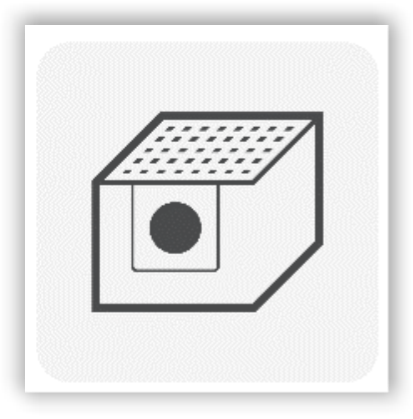
The next item in the data tree is the hydraulics. In this section, we can input and modify the physical elements that make up the project. SSA operates under a subbasin-node-link network model, as illustrated by the graphic below.

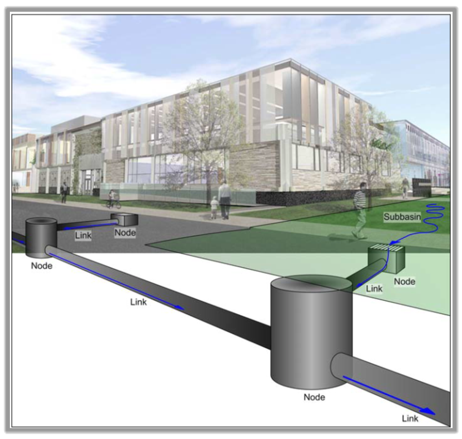
 Source: SSA user manual

SSA Nodes

In SSA nodes are the points where links connect. Since SSA uses a Subbasin-node-link-node model, links are required to connect to a node on both ends. Nodes include Junctions (mostly manholes), Storage Nodes (like ponds), Inlets, Flow diversions, outfalls, and external Inflows.

3.4.1.1                Junctions 

Junctions are typically used to model manhole structures.

But SSA uses a node-link-node model, so Junctions are also used simply as computation points between links. For example, Junctions would be required at the start and/or end of culverts that have headwalls, end- sections, or simply open-ended pipe without a real structure.

3.4.1.2                Storage Nodes

Storage nodes are features that are used to provide storage. They are typically used to represent ponds and other detention facilities. We will see how to use them later to model the pond in our subdivision.

3.4.1.3                Inlets

Stormwater Inlets can represent many different inlet types, including FHWA generic types, as well as inlets manufactured by specific vendors. Specifications will need to be selected to define the type, size, and location of the inlet, invert and rim elevations, and roadway gutter specifications. The inlets on grade (as opposed to in a sag) will require bypass links to be specified in order to route any over-capacity flows past the inlet.

3.4.1.4                Flow diversion

These are structures that we can use anytime we need to split or regulate flows. They are particularly useful in combined sewers.

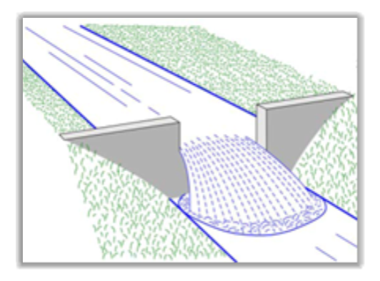
3.4.1.5                     Outfalls 

An Outfall is another type of node element that exists at the end of a network. They are the final item of a pipe run.  Usually, only a single conveyance system or catchment connects to an outfall. They offer several options for simulating the boundary conditions.

SSA Links

The second type of hydraulic element is the link element, which is mostly conveyance types of elements, such as pipes, channels, pumps, orifices, weirs, and outlets.

3.5.1.1                     Conveyance Links 

Conveyance links can model pipes, culverts, channels, or direct connections between nodes.

 

3.5.1.2                     Pumps

Pumps are links used between nodes, whenever we need to lift water.

 

3.5.1.3                     Orifices

Orifices are links that we will use as flow regulation devices. As we will see in the example of the Pre Vs. Post analysis, we will use an orifice to throttle the post development peak flows.

3.5.1.4                     Weirs

Like orifices, weirs can also be used for flow control. They are often used in combination with orifices. In those cases, usually, the orifice is used for low flows, and the weir is used to convey high flows (anything above the 100-Year flood).

3.5.1.5                     Outlets

Outlets are another flow control device (typically from storage nodes). We should not confuse them with outfalls. Outfalls are Nodes while outlets are Links. They are typically used to control outflows from storage nodes (e.g., Detention ponds). They offer the additional capability for managing head vs. discharge data, similar to pump curves but with more options.

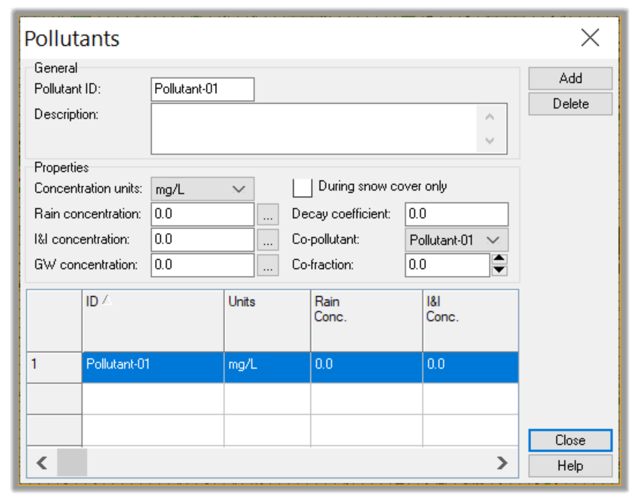
SSA Water Quality

The next line in the data tree is the quality section. In addition to being a very robust water quantity analysis tool, SSA can also perform urban stormwater quality modeling. This is particularly important as more and more permitting authorities require a quality analysis component for each land development project. The water quality module allows us to design and analyze projects with BMP modules such as rain gardens, green roofs, rain barrels, bioswales, dry detention ponds, wet ponds, retention ponds, wetlands, and more.

Using this section, we can perform a water quality analysis taking into account different types of pollutants and land types.

SSA Others

The last item of the data tree is the Others section. In this section, we can dynamically control the on/off status of pumps using the specified STARTUP DEPTH and SHUTOFF DEPTH entries, or by using user-defined rules that we specify in the Control Settings dialog box. For example, we can use control rules to simulate variable speed drives that modulate the pump flow.

Another thing we can do in this section is to input the sanitary flow time patterns. It is very easy to forget the sanitary part in SSA because a majority of users utilize the software only for Stormwater Analysis.

We should keep in mind that SSA allows us to perform a complex sanitary sewer analysis that sizes pipes, controls the flow rules, and manages the patter

If we click on the add button, we can display a new sanitary (dry weather flow) time pattern, select and edit a different time pattern. We can see in this example that we have peak sewer usage early morning between 6am and 8am and in the evening between 6pm and 8pm, when most people are home. We can tweak that by changing the multipliers depending on our local realities.

This concludes the section of the data tree.  Next up is the SSA menu bar.